Monocular Visual Odometry

github:  https://github.com/Juhyung-L/visual_odometry

Visual odometry is the process of estimating the change in position of a robot by processing the image frames from a moving camera. It works by taking individual frames from a prerecorded video or live feed and putting it through a processing pipeline.

The first step in the visual odometry pipeline is feature detection. A feature in an image is a point in the image that can be easily identified in multiple views of the same scene. 

Figure 1: Features extracted from image of a chapel. Each colored circle is a feature.

These two images are pictures of the same building taken from two different view points. There are parts of the building that can easily be identified in both pictures. For example, the three arches on the bottom floor or the circular pattern at the center of the building. For the human brain, features are usually encoded as whole structures just as I have listed above, but they are points for computers and they are identified using mathematical techniques involving the pixel color values.

There are a variety of different feature detection techniques (SIFT, SURF, FAST, BRIEF, ORB, etc), each with its own mathematical definition of what constitutes a feature and the algorithm to detect them. A popular choice for visual odometry is ORB and SIFT. Although these techniques are different, they all accomplish the two same tasks: detecting a feature and storing its pixel coordinate as well as its descriptor.

OpenCV provides the implementation for SIFT feature detector.

A descriptor of a feature is information that will help the feature-matching algorithm to determine which feature from one image corresponds to a feature in the other image. For the human brain, descriptors are in the form of "three arches on the bottom floor" or "circular window at the center". The SIFT technique on the other hand, encodes the pixel values of the 16x16 pixels around the feature point as the descriptor.

Figure 2: Features matched between two pictures of the same building taken from different locations.

The second step in the visual odometry pipline is the feature matching. This step is self-explanatory: features from image 1 are matched to features on image 2 . Like feature detection techniques, there is a variety of different feature matching techniques. In this project, I used the FLANN matcher.

fbm->knnMatch(frame.desc, prev_frame.desc, matches, 3);
// Lowe's ratio test to remove bad matches
for (size_t i=0; i<matches.size(); ++i)
{
    if (matches[i][0].distance < 0.8*matches[i][1].distance) // a good best match has significantly lower distance than second-best match
    {
        matched_kps.push_back(frame.kps[matches[i][0].queryIdx].pt);
        matched_idx.push_back(matches[i][0].queryIdx);
                    
        prev_matched_kps.push_back(prev_frame.kps[matches[i][0].trainIdx].pt);
        prev_matched_idx.push_back(matches[i][0].trainIdx);
    }
}

Lowe's ratio test removes bad matches by comparing the distance(distance is a measure of how good the match is and lower means better match) to the first match and the second match. This test utilizes the fact that good matches usually have significantly lower distances for their first match.

With the feature detection and matching done, we now use techniques in multi-view geometry to extract useful information from these features.

The third step in the pipeline is finding the relative pose of the two cameras using the matched features. This is the source of the odometry information: calculating the relative pose of the cameras in subsequent image frames is estimating the change in pose of the camera as the vehicle moves around. 

In the world of multi-view geometry, there is a special matrix called the essential matrix. Given the following diagram,

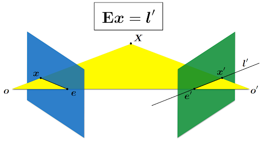
Figure 3:  Relationship between the essential matrix and epipolar lines.

the essential matrix maps a point on one image to a epipolar line on the other image. Epipolar line is a line that connects the an image point to an epipole, which is the position of the second camera as seen from the first camera. This is useful when matching points between two images. In order to match the point x on image 1 to a point on image 2, you only need to search along the epipolar line on image 2 l'. However, we already have a bunch of matched points between two images, which were found using feature detection and matching. With this information, we can work backwards to find the essential matrix.

The reason for calculating the essential matrix is because the relative poses of the cameras are encoded within the matrix. It should be noted here that this process ESTIMATES the essential matrix as we are using points that were matched using a probabilistic method, meaning some matched point pairs are incorrect. Additionally, estimating the essential matrix requires the camera's intrinsic matrix K, which encodes the properties of the camera.

The generalization of the essential matrix to uncalibrated cameras(cameras with unknown K) is the fundamental matrix. However, you cannot directly recover the relative poses from a fundamental matrix. 

Again, OpenCV has a function to do the calculations for you.

E = cv::findEssentialMat(prev_matched_kps, matched_kps, K, cv::FM_RANSAC, 0.9999, 3, 1000, inlier_mask);

With the essential matrix estimated, you can calculate the relative pose of the cameras. With the first camera set to origin of the world frame, all subsequent camera positions are the result of the motion of the camera.

There are two major caveats. Firstly, calculating the change in pose using the essential matrix leaves you with two possible rotations matrices and two possible translation vectors, which produce a total of four possible transformations and only one of these is correct. This ambiguity arises from the physical limitation of trying to determine change in 3D pose using an image, which is inherently 2D.

Figure 4: Ambiguity in pose estimate calculated using the essential matrix.

Luckily, OpenCV's recoverPose() function takes care of this ambiguity and returns the correct pose.

The second caveat is that the estimated translation is also scale-ambiguous, meaning the direction of motion is estimate-able, but not magnitude of the motion. For this reason, OpenCV's recoverPose() function returns the translation vector as a unit vector. This is a major shortcoming of feature-based visual odometry and it is the reason why they are most often used in conjunction with other sensors, such as the IMU or depth sensors, to overcome the scale ambiguity. 

For this project, I opted to use the ground-truth data provided by the KITTI dataset to find the scale of the translation

// get the scale of translation from ground truth
cv::Vec3d true_translation(true_poses[pose_idx](0), true_poses[pose_idx](1), true_poses[pose_idx](2));
double estimated_dist = cv::norm(cv::Vec3d(frame.T(0, 3), frame.T(1, 3), frame.T(2, 3)));
double true_dist = cv::norm(true_translation);
double correction_factor = true_dist / estimated_dist;

frame.T(0, 3) *= correction_factor;
frame.T(1, 3) *= correction_factor;
frame.T(2, 3) *= correction_factor;

Results

Figure 5: Result of the odometry.

The odometry estimation was extremely inaccurate. The estimated path did not resemble the ground-truth path at all and it went off into the sky instead of remaining flat on the ground.

I think the major factor that caused this huge accumulation of error is because of this code.

// apply the translation only if the inlier_count is greater than the threshold
if (inlier_count < min_recover_pose_inlier_count)
{
    estimated_poses.push_back(getPoseFromTransformationMatrix(frame.T)); // append current pose without applying the transform
    return;
}

There were some frames within the video where only a small number of features were detected. In these frames, calculating the pose change yielded extremely inaccurate results (change in position by a factor of few hundred units). To fix this issue, I set a constant integer variable (min_recover_pose_inlier_count) to skip all frames with insufficient numbers of features. Although this method prevented the odometry from blowing up, it still added a significant amount of error over time as more and more frames were skipped.

Figure 6: Error measured in position (x, y, z) and orientation (x, y, z, w) over time.

The error graph was calculated by taking the difference between the ground-truth pose and the estimated pose. The translation errors were obtained by subtracting the x, y, and z components. and the orientation errors were obtained by subtracting the x, y, z, and w components (quaternion).

Tweaking the parameters from any of the image-processing steps (feature extraction, feature matching, and pose estimation) could have reduced the error, but it is not a generalized solution. More general solutions for reducing error in visual odometry systems are loop closure and pose-graph optimization.

Video Footage