Stereo Visual Odometry (with Bundle Adjustment)
Visual odometry is the process of estimating a camera's position by processing the individual images taken from a moving camera. It can be performed with different types of cameras: monocular (single camera), stereo (two cameras), depth (camera with depth info). In this blog, I will explain the inner workings of a visual odometry system for a stereo camera setup.
Figure 1: My implementation of stereo visual odometry.
A stereo camera is a pair of cameras facing the same direction that are separated by a known distance.

Figure 2: Stereo camera setup.
Unlike a monocular camera, the stereo camera can estimate the depth of a pixel on an image using a technique called triangulation. This is similar to how humans can sense how far away an object is using both eyes. The system also includes bundle adjustment, a non-linear error minimization technique used to reduce the accumulation of error in the pose estimates. I hope to see improved accuracy in the pose estimate compared to the monocular version.
Visual Odometry Pipeline

Figure 3: Stereo visual odometry pipeline.
Step 1: Detect Features in Left Image
Features are extracted from the left image using FAST (Features from Accelerated Segment Test) feature detector in OpenCV.
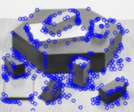
Figure 4: FAST features extracted from a picture of polygon blocks (each blue circle is a feature).
Step 2: Match Features in Right Image
Features in the left image are matched to features in the right image. In other words, if in the left image you detected a feature on a tree, you need to detect the same feature in the right image and know that those two features correspond to each other. This can be done using the calcOpticalFlowPyrLK function in OpenCV.

Step 3: Triangulate Features
Once you know the correspondence of features in the left and right image pair, you can use triangulation to find the 3-dimensional location of the feature.
Brief Explanation of Triangulation:
Given:
- X (3D point)
- P (camera projection matrix)
- x (2D projection of X onto image plane)
The relationship between x and X is x = PX. This means projecting X onto the image plane with the projection matrix yields x. If you only have one x and you try to solve for X, you get a line with infinitely many solutions.

Figure 6: Solving for 3D point with one 2D image point.
When you have two or more x's, you can solve for X by getting the intersection between the two lines.

Figure 7: Solving for 3D point with two 2D points.
However, sensor measurements are usually noisy and there will not be an intersection most of the time. Hence, the point with the minimum distance to both lines is selected.
Step 4: Match Features in Next Left Image
The features that were triangulated in the previous step is found in the next left image using the function calcOpticalFlowPyrLK in OpenCV.
Step 5: Estimate Pose of Next Left Image
Now that we have the correspondence between 2D features and their 3D position, we can use find the pose of the image plane by minimizing the reprojection errors of the 3D points. This is exactly what the function solvePnRRansac() does in OpenCV.
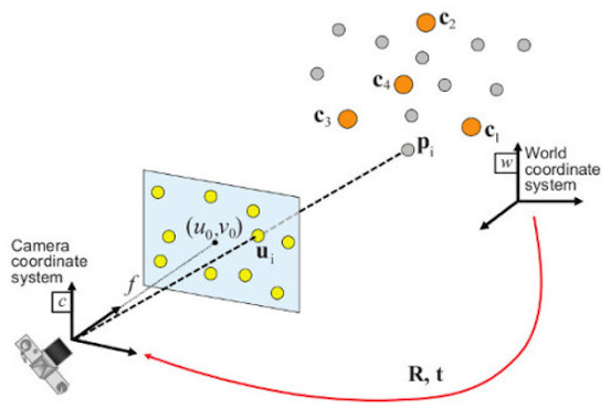
Figure 8: Persepective-n-Point pose estimation.
The pose with the minimum difference between the 2D points (observation) and reprojections (actual) is the pose of the image plane. Check out https://docs.opencv.org/4.x/d5/d1f/calib3d_solvePnP.html for more information on how the function works.
Result (without Bundle Adjustment)
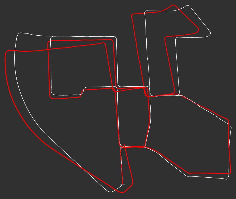
Figure 9: Stereo visual odometry (without bundle adjustment) on KITTI dataset. Red line=odometery and white line=ground truth.

Repeating steps 2 - 5 will give a pretty accurate pose estimate for the first minute or so. However, because the pose estimate is calculated for each consecutive image pair and added to the total pose estimate, the small errors in each estimate build up over time. This is called odometric drift. To correct this drift, a technique called bundle adjustment is used.
Bundle Adjustment
Figure 11: Performing bundle adjustment on pose (arrow) and 3D feature (circle) estimates. The green markers represent estimates and red markers represent ground truth. The inaccurate estimates are corrected by minimizing the reprojection errors of the 3D features onto the image planes.
Bundle adjustment is an optimization process of refining the poses of multiple cameras and 3D features such that it yields the lowest reprojection error. Other parameters, such as camera intrinsics and distortion coefficients, can be part of the variables being optimized, but I used the KITTI dataset which provided me with accurate intrinsics and undistorted images. Hence, I did not include them in the optimization. Additionally, bundle adjustment is a non-linear optimization problem and implementing such feature from scratch requires mastery of various fields of mathematics as well as programming. So, I used a off-the-shelf optimization library called Ceres Solver.
Result (with Bundle Adjustment)

Figure 12: Stereo visual odometry (with bundle adjustment) on KITTI dataset. Red line=odometery and white line=ground truth.

Figure 13: Side view of figure 12

Figure 14: Bottom view of figure 12
As shown in figure 12, bundle adjustment significant increases the accuracy of the pose estimate. However, the estimate still has a large margin of error in terms of the elevation of the camera as shown in figures 13 and 14. This is an area for future improvement.


Comments
Post a Comment